Radial FTLE Structure. What the Data Actually Reveals

Something say before ...

✅ Our radial decomposition worked.

But it also revealed a surprise that sharpens (and slightly corrects) our temporary theory:

Depth in narrow nets is not creating “directional ridges” (anisotropy in \theta); it is creating a radially symmetric boundary bump (localization in r). Meanwhile the big angular anisotropy is actually coming from N=10,L=2, and it lives mostly outside the GT boundary.

Let's go point by point.

1) What the mean profile $m (r) = E_{θ} [λ_{T} (r, θ)]$ says

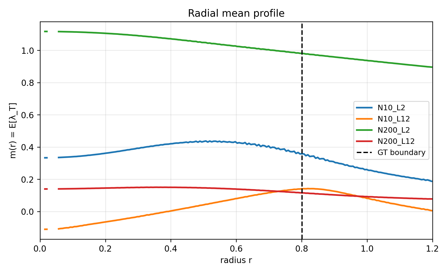
(N=200, L=2) green 🪀: “high baseline, gently decreasing”

m(r) is large everywhere and decreases smoothly with r.
No peak at the GT boundary $r_{*} \approx 0.8$ .

Interpretation: sensitivity is dominated by a global smooth component (not boundary-localized).

(N=200, L=12) red 🧧: “depth crushed the baseline”

Same shape as green (smooth, monotone-ish), but the magnitude is much smaller.
Still no boundary peak.

This is exactly our “wide+deep homogenization” story: depth doesn’t create localization; it reduces/averages/quenches the field.

This aligns with your earlier observation: RA shifts a bit, but $G_{λ}$ collapses.

(N=10, L=2) blue 🌀: “peak is inside, not at boundary”

The hump peaks around r\sim 0.5, not at $r_{*} \sim 0.8$ .
At the boundary, m(r) is already decreasing.

Interpretation: this is not boundary-focused geometry. It’s more like “interior sensitivity” (could be saturation/activation geometry effects, or spurious finite-width structure).

(N=10, L=12) orange 🍊: “boundary bump appears”

This is the most important qualitative feature:
m(r) rises up to near the GT boundary, peaks very close to r_*, then drops.

This is exactly the kind of “decision-boundary localization” we were hoping to see from the rich/feature-learning corner.

So: ✅ expected and confirmed (at least in the radial mean sense).

2) What the angular variance profile $v (r) = {Var}_{θ} [λ_{T} (r, θ)]$ says

This plot is even more diagnostic than the mean.

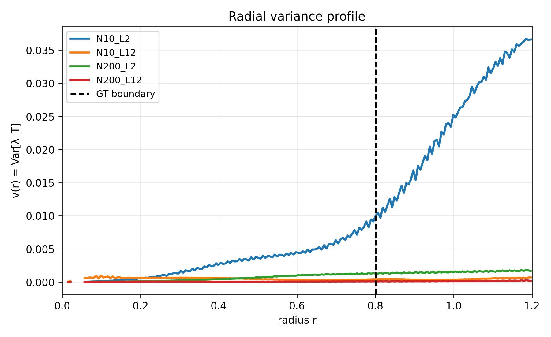
Huge surprise: N=10,L=12 has tiny $v (r)$

Orange is near ~0 everywhere.

Meaning: the FTLE field at $N = 10, L = 12$ is almost perfectly rotationally symmetric (within your binning/estimation noise).

So if we were imagining “ridges” as directional structures, they are not showing up here.

Instead, what you have is radial localization without angular anisotropy:

a “ring bump,” not “ridges”.

This is a conceptual refinement:

“ridge-rich” (directional) is not the only way to be geometrically meaningful.
You can have a boundary-localized ring that is isotropic.

The dominant angular anisotropy is N=10,L=2 blue — and it grows outside the boundary

Blue explodes for $r > 0.8$ .

Interpretation: this is likely finite-width noise / directional instability in the exterior region, not “useful ridge geometry” tied to the decision boundary.

This also explains why $G_{λ}$ can be large at $N = 10, L = 2$ : it’s coming from anisotropy/tails far from the boundary, not from meaningful boundary concentration.

Wide nets (green/red) have tiny $v (r)$

As expected: width self-averages away angular structure.

3) Tier-III scalar metrics confirm the same story

label	width	depth	gain	base_lr	spike_height	fwhm	tail_stat
N10_L2	10	2	1.0	0.05	0.0256	0.686	0.1865
N10_L12	10	12	1.0	0.05	0.2510	0.743	0.1279
N200_L2	200	2	1.0	0.05	-0.136	0.0	0.1415
N200_L12	200	12	1.0	0.05	-0.024	0.0	0.0593

From our tier3_scalar_metrics.csv (gain=1.0, lr=0.05):

Spike height $H = m (r_{*}) - m (r_{c e n t e r})$
- $N 10, L 12 : 0.251$ (big!)
- $N 10, L 2 : 0.026$ (tiny)
- $N 200, L 2 : - 0.136, N 200, L 12 : - 0.024$ (boundary lower than center)

✅ This quantitatively certifies what we saw by eye:

Only N10,L12 produces a strong boundary-localized mean bump.

Tail statistic $T = Q_{0.95} (λ) - Q_{0.5} (λ)$
- $N 10, L 2 : 0.186$ (largest)
- $N 200, L 2 : 0.141$
- $N 10, L 12 : 0.128$
- $N 200, L 12 : 0.059$

⚠️ This is subtle: the largest tail is not $N 10, L 12$ but $N 10, L 2$ , consistent with the variance plot (blue has crazy angular variance/tails outside boundary).

This tells us an important scientific point:

A global tail metric over the whole grid is dominated by “where the instability lives,” not necessarily “where the decision boundary is.”

So your tail metric is good, but you should also compute a boundary-conditioned tail (see next section).

4) Is it “as expected”?

Yes, the core hypothesis is supported:

Wide+deep → smooth, uniform, quenched FTLE field (both $m$ and $v$ small-ish; especially $v$ ).
Narrow+deep → decision-boundary localization shows up clearly in $m (r)$ .

But we must correct one expectation:

We previously leaned toward “rich ⇒ directional ridges ⇒ large v(r).”

Your data says:

N10,L12 is “rich” by RA/KA, and it shows boundary localization in $m (r)$ ,
but it is not ridge-y in the angular sense (tiny $v (r)$ ).

So the refined temporary theory is:

Feature motion (RA/KA) can create boundary-localized sensitivity as a ring (radially isotropic), not necessarily as directional ridges.

Directional ridge-ness (anisotropic v(r)) is a separate phenomenon and may be strongest in “noisy finite-width” settings (like N10,L2) rather than in the clean rich regime.

This is actually a stronger and cleaner story.