One-Dimensional System

Fixed Point

Consider the one-dimensional system:

The fixed point found by setting $\dot{x}=0$. For the fixed point $x^{\ast }$. We will use it for determining the stability.

Example

For equation $\dot{x}=x^2-1$, we have it's plot here:

---
title: x' = x^2-1
xLabel: x
yLabel: x'
bounds: [-2,2,-2,2]
disableZoom: false
grid: true
---
f(x)=x^2-1
g(x)=0

The left fixed point $x^{\ast }=(-1,0)$ is a stable point, while the right FP$(1,0)$ is unstable.

Linear Stability Analysis

In order to know the behavior around fixed point linearization is a great method to analyze.

Let $x^{\ast }$ be a fixed point, and let $\eta (t)=x(t)-x^{\ast }$ be a small perturbation away from $x^{\ast }$. To see whether the perturbation grows or decays, we derive a differential equation for $\eta$. Differentiation yields

since $x^{\ast }$ is constant. Thus $\dot{\eta }=\dot{x}=f(x)=f(x^{\ast }+\eta )$. Now using Taylor’s expansion we obtain

where $O({\eta }^2)$ denotes quadratically small terms in $\eta$. Finally, note that $f(x^{\ast })=0$ since $x^{\ast }$ is a fixed point. Hence

Now if $f^{\prime }(x^{\ast })\ne 0$, the $O({\eta }^2)$ terms are negligible and we may write the approximation

This is a linear equation in $\eta$, and is called the linearization about x*. It shows that the perturbation:

Potentials

There’s another way to visualize the dynamics of the first-order system: potential $V(x)$ is defined by

Consider the relation between potential and time $V(x(t))$, by using chain rule we have

since $\dot{x}=f(x)$, we obtain

The equilibrium point happens at $dV/dx=0$, the $V$ remains constant. Since $dV/dx=0$ implies $\dot{x}=0$.

Example

Graph the potential for the system $\dot{x}=x-x^3$, and identify all equilibrium points.

$\mathbf{\text{Solution:}}$ Solving $-dV/dx=x-x^3$ yields

Once again we set $C=0$. Figure shows the graph of $V$. The local minima at $x=\pm 1$ correspond to stable equilibria, and the local maximum at $x=0$ corresponds to an unstable equilibrium.

---
title: V(x)-Potential
xLabel: x
yLabel: V(x)
bounds: [-2,2,-0.5,1]
disableZoom: false
grid: true
---
f(x)=-0.5x^2+0.25x^4

Bifurcations

Saddle-Node

Typical Form:

Splitting into two branches.

Transcritical Bifurcation

Normal Form:

Some people say that an exchange of stabilities has taken place between the two fixed points.

Pitchfork Bifurcation

This bifurcation is common in physical problems that have a symmetry.

Supercritical Pitchfork Bifurcation

Normal Form:

Note that this equation is invariant under the change of variables $x\to -x$.

One stable splitting two stable and one unstable.

Subcritical Pitchfork Bifurcation

Normal Form:

One stable and two unstable to one stable.

Dimensional Analysis

Non-dimensionalization

Differential equations that show up in modeling “real world situations” usually have many constants in them. Often one can reduce the number of constants in a problem by choosing the right units for the various quantities in the problem. In the other words, we can convert the variables to ratio that has no unit to analyze multiple different coefficient problems.

We define a dimensionless time $\tau$ by

where $\tau$ is dimensionless time, $t$ is dimensional time, $T$ is characteristic time scale. We need to choose $T$ very carefully to do the non-dimensionalization.

Timescale

$\lambda$ is the rate of growth. $1/|\lambda |$ is timescales of growth.

Example 1

Suppose that a quantity $x(t)$ changes in time according to the ODE

The coefficients $a$, $b$, and $c$ must all have different units, otherwise we could not add the terms $a$, $bx$, and $c{x}^2$.

To simplify the equation we choose a constant value for $x$, let's say $x_0$, and we let this value be our unit. The ratio

has no units. In the same way we can pick a unit of time $t_0$ and introduce the quantity

which also has no units.

The quantities $\xi$ and $\tau$ are nondimensionalized versions of our original variables $x$ and $t$. The point of nondimensionalization is that we can now derive a differential equation for $\xi$ and $\tau$, and then afterwards figure out which choice of the units $x_0$ and $t_0$ simplifies things most.

In this example we substitute

which leads to

by the chain rule, and

by direct substitution. The differential equation (1) for $x$ and $t$ is therefore equivalent with

and thus

At this point we choose $x_0$ and $t_0$. We can try to make the constant term and the coefficient of $\xi$ both equal to 1. If $a\ne 0$ and $b\ne 0$ then this is possible provided we choose

The coefficient of ${\xi }^2$ then becomes

and we get the following differential equation for $\xi$ as a function of $\tau$:

This is a nondimensionalized version of equation (1). Note that instead of three undetermined parameters $(a,b,c)$ it only has one parameter, namely $\alpha$.

Example 2

The Logistic equation:

where $N$ is population, $t$ is time, $r$ growth rate, $K$ carrying capacity.

The non-dimensionalize term:

Thus, we have

when $T=1/r$ and $N_0=K$.

Two-Dimensional System

General form

$2D$ system:

Example

Let $x=\varphi$, $y=\dot{\varphi }$, then we have

Linear form

where $a,b,c,d$ are $\mathbb{R}$. Let $\mathbf{x}=\left(\begin{array}{c}x\\ y\end{array}\right)$ , $A=\left(\begin{array}{cc}a& b\\ c& d\end{array}\right)$, so we have $\dot{\mathbf{x}}=A\mathbf{x}$.
The fixed points: when $\dot{x}=\dot{y}=0$ or $\dot{\mathbf{x}}=\mathbf{0}$.

Uncoupled System

Consider the system

Notice $\{\begin{array}{l}\dot{x}=ax\\ \dot{y}=-y\end{array}$ = $\{\begin{array}{l}x=x_0{e}^{at}\\ y=y_0{e}^{-t}\end{array}$ the trajectory is different and depends on $a$:

Classified these cases: $(a)$ Stable node, $(b)$ Stable star,
$(c)$ stable node, $(d)$ line of fixed points, $(e)$ saddle point

Stability Technology

When $x^{\ast }$ is a fixed point:

• $x^{\ast }$ is attracting if all trajectories near $x^{\ast }$ approach it as $t\to \mathrm{\infty }$.
• $x^{\ast }$ is globally attracting if all trajectories approach it as $t\to \mathrm{\infty }$.
• $x^{\ast }$ is Lyapunov stable if all trajectories that start sufficiently close to $x^{\ast }$ remain close for all time
  There are three cases to help understand:

1. Attracting but not Lyapunov Stable

2. Lyapunov Stable but not attracting

3. Attracting and Lyapunov is Stable Start $(b)$ case.

General Linear System

Consider following form

Note: The straight-line trajectories is if $\mathbf{x}(0)=\left(\begin{array}{c}{x}_0\\ 0\end{array}\right)$ then $\mathbf{x}(t)=\left(\begin{array}{c}x(t)\\ 0\end{array}\right)$ which is stays on $x$-axis.

Now let's generalize this idea. Let's guess $\mathbf{x}(t)=e^{\lambda t}\mathbf{v}$ , hence $\lambda$ is the growth rate and $\mathbf{v}$ is the direction of growth (the vector).

So, $\dot{\mathbf{x}}(t)=A\mathbf{x}$ implies $\lambda e^{\lambda t}\mathbf{v}=e^{\lambda t}A\mathbf{v}$ and

So, $\mathbf{v}$ is an eigenvector and $\lambda$ is an eigenvalue. $\mathbf{x}(t)=e^{\lambda t}\mathbf{v}$ is an eigensolution.

2D Eigenvalues

Definition

Then the this singular matrix has determinant zero:

Thus, $\lambda =\frac{{\tau }^2\pm \sqrt{{\tau }^2-4\mathrm{\Delta }}}{2}$, $\tau =a+d$, and $\mathrm{\Delta }=ad-bc$.
The eigenvectors are when you plug the eigenvalues back to the original form.

Note: $\tau ={\lambda }_1+{\lambda }_2$, $\mathrm{\Delta }={\lambda }_1{\lambda }_2$

System form

When ${\lambda }_1\ne {\lambda }_2$ the general form of the system is

Example

For linear system:

we have $A=\left(\begin{array}{cc}1& 1\\ 4& -2\end{array}\right)$ and ${\mathbf{x}}_{\mathbf{0}}=\left(\begin{array}{c}2\\ -3\end{array}\right)$ . Then the $\tau =1-2=-1$, $\mathrm{\Delta }=-2-4=-6$, so ${\lambda }^2+\lambda -6=0$ gives ${\lambda }_1=2$ and ${\lambda }_2=-3$.
So, by plugging ${\lambda }_{1,2}$ backs to determent equation, we have

By set $t=0$ I get $c_1=c_2=1$. Therefore the general solution is

Phase diagrams & Fixed Points

Normal Cases

The different $\lambda$ are right below:

$(a)$ $0<{\lambda }_1<{\lambda }_2$ (top left), $(b)$ ${\lambda }_1=0<{\lambda }_2$ top right, $(c)$ ${\lambda }_1<0<{\lambda }_2$ (down left), $(d)$ ${\lambda }_1<{\lambda }_2<0$ (down right).

Remark: When ${\lambda }_1<{\lambda }_2=0$ is the a line of stable FPs(reverse arrow for $(b)$).

Spacial Cases

When ${\lambda }_1={\lambda }_2$, there are two possible cases:

1. There are two independent eigenvectors ${\mathbf{v}}_1,{\mathbf{v}}_2$.
   This will lead the $A$ to $\left(\begin{array}{cc}\lambda & 0\\ 0& \lambda \end{array}\right)$ , so the diagram would be Star node. If $\lambda <0$, stable star. If $\lambda >0$, unstable star. When $\lambda =0$, all points are fixed points.
2. There is only one eigenvector.
   Only eigenvector would be $A=\left(\begin{array}{cc}\lambda & b\\ 0& \lambda \end{array}\right)$ thus the eigenvector is $\left(\begin{array}{c}b\\ 0\end{array}\right)$ . This is called degenerative node

This graph is with $b>0$ and $\lambda <0$.

If ${\tau }^2-4\mathrm{\Delta }<0$ we have ${\lambda }_{1,2}=\alpha \pm i\omega$ where the $\alpha$ is complex conjugate eigenvalues.

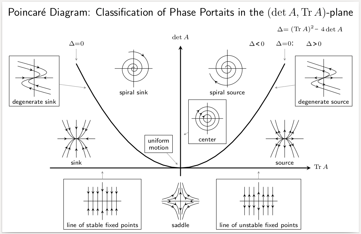
Poincare Diagram

Nullclines

The nullclines are designed as the lines along with $x,y$ not changing (i.e. $\dot{x}=0$, $\dot{y}=0$). For example, when $\{\begin{array}{l}\dot{x}=0\\ \dot{y}=0\end{array}$ , we have $x+e^{-y}=0$ and $y=0$. so it will look like this.

Note:

1. Not trajectory
2. Nullclines cross at fixed point
3. Trajectories are either horizontal $(y=0)$ or vertical $(x=0)$ when it at numllclines

System Uniqueness Theorem

Consider the IVP(initial value problem). If $f$ and it's partial derivative (Jacobian matrix) are continuous for all $\mathbf{x}$ in an open-connected set $D\subseteq {\mathbb{R}}^2$ contain of $x_0$, hence the trajectory has only one solution. No cross point.

Linearization

Consider a general linear system and it's fix point $(x^{\ast },y^{\ast })$, the perturbation is $\{\begin{array}{l}x(t)=x^{\ast }+u(t)\\ y(t)=y^{\ast }+v(t)\end{array}$. Now consider $f(x,y)=f(x^{\ast }+u,y^{\ast }+v)$ we can use Taylor Expansion to get below:

So $A=\left(\begin{array}{cc}{f}_x& f_y\\ g_x& g_y\end{array}\right)$ under fixed point $(x^{\ast },y^{\ast })$.

When $\lambda =a+bi$

Reversible

Many mechanical systems have time-reversal symmetry. This means that their dynamics look the same whether time runs forward or backward. For example, if you were watching a movie of an undamped pendulum swinging back and forth, you wouldn’t see any physical absurdities if the movie were run backward.

The system is reversible if invariant under the mapping of $(t,x)\mapsto (-t,R(x))$
Time-reversible $(t,x,y)\mapsto (-t,x,-y)$. We have symmetric along the $x=0$ with different direction of arrows. In other words, for 2D system $\{\begin{array}{l}\dot{x}=f(x,y)\\ \dot{y}=g(x,y)\end{array}$ it such that $f$ is odd in $y$ and $g$ is even in $y$ ,aka $f(x,-y)=-f(x,y)$ and $g(x,-y)=g(x,y)$.

Invariant under $(t,x,y)\mapsto (t,-x,y)$ give us it is symmetric along with $y=0$ but the direction of arrow at not change.

Note: Any mechanical systems have time-reversal symmetry. i.e. $m\ddot{x}=F(x)$. is symmetric under time reversal.

Polar Coordinate

Sometimes we cannot justified the centre case, we might trans the system into polar system to analyze. The following example:

Waiting to be filled Week 7 Class 18

Trans to polar system. Let $(x,y)=(r\cos \theta ,r\sin \theta )$. Then using

For polar system we can determine the limit cycle by let $\dot{r}=0$ then solved for $r$. If there exist $r>0$ that means there exist circular limit cycle. We also can determine what is the behavior around limit cycle by analyzing the vector field around fixed point for $\dot{r},r$.

Wolfram Code

f[x_, y_] := y
g[x_, y_] := -a*y*(x^2 + y^2 - 1) - x


x0 := r*Cos[\[Theta]]
y0 := r*Sin[\[Theta]]

fr[x_, y_] := (x*f[x, y] + y*g[x, y])/r
fth[x_, y_] := (x*g[x, y] - y*f[x, y])/r^2

rp := Simplify[fr[x0, y0]]
thp := Simplify[fth[x0, y0]]

rp
thp

Poincaré–Bendixson Theorem

1. $R$ is a closed, bounded subset of the plane;
2. $\dot{x}=f(x)$ is a continuously differentiable vector field on an open set containing $R$;
3. $R$ does not contain any fixed points; and
4. There exists a trajectory $C$ that is "confined" in $R$, in the sense that it starts in $R$ and stays in $R$ for all future time.
   Then either $C$ is a closed orbit, or it spirals toward a closed orbit as $t\to \mathrm{\infty }$. In either case, $R$ contains a closed orbit.

Note. The problem of this question is find the trapping region. Here is an example showing how to make it.

Example

Given a system:

Consider $r_1$ as the radius for inner circle, $r_2$ as the radius for outer circle. Then for $r_1$ must such that $\dot{r}>0$ and for $r_2$ must such that $\dot{r}<0$. Thus we have

Thus, to hem in the limit cycle as tightly as we can. For instance, we could pick
$r_{\text{min}}=0.999\sqrt{1-\mu }$. (Even $r_{\text{min}}=\sqrt{1-\mu }$ works, but more careful reasoning is required.) By a similar argument, the flow is inward on the outer circle if $r_{\text{max}}=1.001\sqrt{1+\mu }$.

Conservation Systems

The energy is often called a conserved quantity, a constant of motion, or a first integral. Systems for which a conserved quantity exists are called conservative systems.

Conservative

$\dot{x}=f(x)$ is a conservative system. if there exist a real valued function that is constant along trajectories, but non-constant on every open set.

Linear centre implies nonlinear centre.

Process

Let's explain with example. Newton's Second Law is a classic conservation system: $m\ddot{x}=F(x)$. By potential energy we have $F(x)$ force as $F(x)=-\frac{dV}{dx}$ where $V(x)$ is the potential energy. Then we have $m\ddot{x}+\frac{dV}{dx}=0$. Now the only thing we need to do is integration. By multiplied $\dot{x}=\frac{dx}{dt}$ we have

Thus, $E=\frac{1}{2}m{\dot{x}}^2+V(x)$ is the energy which is a Conserved Quantity. And the $\frac{1}{2}m{\dot{x}}^2$ is the Kinetic Energy and $V(x)$ is Potential Energy in Physics. It is constant along trajectories.

Note: A conservative system cannot have attracting fixed points. (they are circle)

Check Conservative

Consider a polar system $\dot{x}=-\sin \theta -D{x}^2$, $x\dot{\theta }=-\cos \theta +x^2$ . Now check if $E(x,\theta )=x^3-3x\cos \theta$.
\begin{proof}
First take the derivative with respect to $t$

\end{proof}

Theorem

(Nonlinear centers for conservative systems) Consider the system $\dot{\mathbf{x}}=\mathbf{f}\mathbf{(}\mathbf{x}\mathbf{)}$ , where $\mathbf{x}=(x,y)\in {\mathbb{R}}^2$, and $\mathbf{f}$ is continuously differentiable. Suppose there exists a conserved quantity $E(x)$ and suppose that $x^{\ast }$ is an isolated fixed point (i.e., there are no other fixed points in a small neighborhood surrounding $x^{\ast }$). If $x^{\ast }$ is a local minimum of $E$, then all trajectories sufficiently close to $x^{\ast }$ are closed.

Index Theory

The index of a closed curve $C$ is an integer that measures the winding of the vector field on $C$. The index also provides information about any fixed points that might happen to lie inside the curve.

Then at each point $\mathbf{x}$ on $C$, the vector field $\dot{\mathbf{x}}=(\dot{x},\dot{y})$ makes a well-defined angle $\varphi =-\tan (\dot{y}/\dot{x})$ with the positive $x$-axis.

Then the index of the closed curve $C$ with respect to the vector field $\mathbf{f}$ is defined as

Given the ordered directions rotate once counterclockwise as we go in increasing order from vector $1$ to vector $8$. Hence $I_C=+1$. Of course the clockwise is $I_C=-1$. The example of $I_C=+1$ is

Properties

1. Suppose that $C$ can be continuously deformed into $C^{\prime }$ without passing through a fixed point. Then $I_C=I_C^{\prime }$.
2. If $C$ doesn’t enclose any fixed points, then $I_C=0$.
3. If we reverse all the arrows in the vector field by changing $t\to -t$, the index is unchanged (Invariant).
4. Suppose that the closed curve $C$ is actually a trajectory for the system, i.e., $C$ is a closed orbit. Then $I_C=+1$.

Note. The Invariant set means any trajectory that starts in set $A$ stays in $A$ for all time.

Theorem 1

If a closed curve $C$ surrounds $n$ isolated fixed points ${\mathbf{x}}_1^{\ast },\dots ,{\mathbf{x}}_n^{\ast }$, then

where $I_k$ is the index of ${\mathbf{x}}_k^{\ast }$, for $k=1,\dots ,n$.

Theorem 2

Any closed orbit in the phase plane must enclose fixed points whose indices sum to $+1$.

\begin{proof}
Let $C$ denote the closed orbit. From property $(4)$ above, $I_C=+1$. Then Theorem 1 implies $\sum _{k=1}^n{I}_k=+1$.
\end{proof}

Fact

$I_C=+1$: Degenerate, Spiral, Centre, Nodes, Stars.
$I_C=-1$: Saddle.
There is no possible to have closed orbit for those fixed points on the straight-line vector space. Since it will always have cross of two orbit.

Invariant

Invariant lines: Every point along the line are also have same direction.

It could happen on fixed points. Let's looks some example:

Example

Let $A,B,C$ as three fixed point, so there are three linear line $AB,BC,AC$. Assume that they are $y=mx+b$. Then, invariant means $\dot{y}=m\dot{x}$ are consistency on each $y=mk+b$.
You can usually plug $y$ into $\dot{y},\dot{x}$ to see if they match the $\dot{y}=m\dot{x}$.

Also, to know that for $y=x^2$, we want to check $\dot{y}=2x\dot{x}$.

Gradient System

Suppose the system can be written in the form $x=-\mathrm{\nabla }V$, for some continuously differentiable, single-valued scalar function $V(x)$. Such a system is called a gradient system with potential function $V$.

If we want to know if a system is gradient, we need to check the definition. If the $\partial V/\partial x=-f(x,y)$, $\partial V/\partial y=-g(x,y)$. Thus let's explain with an example

Example

For system $\dot{x}=y^2+y\cos x$, $\dot{y}=2xy+\sin y$.
Now we test $\partial V/\partial x=-f(x,y)$ we have

Then we test $\partial V/\partial y=-g(x,y)$ we have

Thus we can find a potential function $V(x,y)=-y^{2}x-y\sin x$ such the conditions. So the system is a gradient system.

Theorem

Closed orbits are impossible in gradient systems.

How to find the Potential function

In 2D, the gradient system such that

Thus, we can use an example to explain it:

Example

Show that there are no closed orbits for the system $\dot{x}=\sin y$, $\dot{y}=x\cos y$.
\begin{proof}
The system is a gradient system with potential function $V(x,y)=–x\sin y$. We can see that the $\partial V/\partial x=-\sin y$, $\partial V/\partial y=-x\cos y$, then we have $\int \partial V/\partial x=-x\sin y$ and $\int \partial V/\partial y=-x\sin y$. Thus we can find there exist a $V(x,y)$ such the condition of gradient system.
\end{proof}

Liapunov Function

consider a system $\dot{\mathbf{x}}=\mathbf{f}(\mathbf{x})$ with a fixed point at ${\mathbf{x}}^{\ast }$. Suppose that we can find a Liapunov function, i.e., a continuously differentiable, real-valued function $V(x)$ with the following properties:

1. $V(\mathbf{x})>0$ for all $\mathbf{x}\ne {\mathbf{x}}^{\ast }$, and $V({\mathbf{x}}^{\ast })=0$. (We say that $V$ is positive definite.)
2. $\dot{V}<0$ for all $\mathbf{x}\ne {\mathbf{x}}^{\ast }$. (All trajectories flow “downhill” toward ${\mathbf{x}}^{\ast }$.)

Liapunov function is a "there exist" statement which means you only find one function that such the conditions then you can say it is Liapunov.

Note. $\dot{V}=0$ means the minimum or maximum stable pr unstable point of the system.

Note. Asymptotic stability means that solutions that start close enough not only remain close enough but also eventually converge to the equilibrium.

Example

For given system $\dot{x}=y-x^3$, $\dot{y}=-x-y^3$.
\begin{proof}
By constructing a Lyapunov function $V(x,y)=a{x}^2+b{y}^2$, we can form a suitable $a,b$ for the system. Then we have $\dot{V}(x,y)=2ax\dot{x}+2by\dot{y}$, by substituting the system we have

When $a=b>0$, we have $\dot{V}(x,y)=-2x^{4}a-2y^{4}b<0$. Thus the system is stable. Since the system is stable, so there is no closed orbits.
\end{proof}

Chaos System

Lorenz Equation

Consider the Lorenz Equation:

Here $\sigma ,r,b>0$ are parameters: $\sigma$ is the Prandtl number, $r$ is the Rayleigh number, and $b$ has no name.

Properties

Nonlinearity

The system has only two nonlinearities, the quadratic terms $xy$ and $xz$.

Symmetry

There is an important symmetry in the Lorenz equations. If we replace $(x,y)\to (–x,–y)$ in system, the equations stay the same. Hence, if $(x(t),y(t),z(t))$ is a solution, so is $(–x(t),–y(t),z(t))$. In other words, all solutions are either symmetric themselves, or have a symmetric partner.

Volume Contraction

The Lorenz system is dissipative: volumes in phase space contract under the flow.

Pick an arbitrary closed surface $S(t)$ of volume $V(t)$ in phase space. Think of the points on $S$ as initial conditions for trajectories, and let them evolve for an infinitesimal time $dt$. Then $S$ evolves into a new surface $S(t+dt)$; what is its volume $V(t+dt)$?

Let $\mathbf{n}$ denote the outward normal on $S$. Since $\mathbf{f}$ is the instantaneous velocity of the points, $\mathbf{f}\cdot \mathbf{n}$ is the outward normal component of velocity.

Hence

so we obtain

Hence

Finally, we rewrite the integral above by the divergence theorem, and get

For the Lorenz system,

Since the divergence is constant, it reduces to

which has solution

Thus volumes in phase space shrink exponentially fast. The important key here is showing $\mathrm{\nabla }\cdot \mathbf{f}<0$ which implies the system is dissipative.

One-Dimensional Map

Fixed Point

The fixed point in one-dimensional map is different from continuity function. The general form of the one-dimensional map is

Thus, we set a point $x^{\ast }$ that is always goes to itself $x^{\ast }=f(x^{\ast })$. And that would be the fixed point.

Stability Analysis

Similar to continuity function, we also using perturbation to analyze it. To determine the stability of $x^{\ast }$, we consider a nearby orbit $x_n=x^{\ast }+{\eta }_n$ and ask whether the orbit is attracted to or repelled from $x^{\ast }$. That is, does the deviation ${\eta }_n$ grow or decay as $n$ increases? Substitution yields

But since $f(x^{\ast })=x^{\ast }$, this equation reduces to

Suppose we can safely neglect the $O({\eta }_n^2)$ terms. Then we obtain the linearized map ${\eta }_{n+1}=f^{\prime }(x^{\ast }){\eta }_n$ with eigenvalue or multiplier $\lambda =f^{\prime }(x^{\ast })$.

The solution of this linear map can be found explicitly by writing a few terms: ${\eta }_1=\lambda {\eta }_0$, ${\eta }_2=\lambda {\eta }_1$, and so in general ${\eta }_n={\lambda }^n{\eta }_0$. If $|\lambda |=|f^{\prime }(x^{\ast })|<1$, then ${\eta }_n\to 0$ as $n\to \mathrm{\infty }$ and the fixed point $x^{\ast }$ is linearly stable. Conversely, if $|f^{\prime }(x^{\ast })|>1$ the fixed point is unstable. In mathematics language

There is a special case when multiplier $\lambda =0$ i.e. $f^{\prime }(x^{\ast })=0$ we call superstable.

Logistic Map

The map is looks like

The fixed points are $x^{\ast }=r{x}^{\ast }(1-x^{\ast })$ which are $x^{\ast }=0$ and $x^{\ast }=1-1/r$. Since we only consider the positive, the second fixed point has range of allowable $r\ge 1$.

By analyzing the stability, we have the multiplier $f^{\prime }(x^{\ast })=r-2r{x}^{\ast }$. Thus we have stability for $x^{\ast }=0$:

and for $x^{\ast }=1-1/r$:

Bifurcation Type

From the map we can easily see that what type at each point:

As we can see, when $r=1$ it is a transcritical bifurcation.

Once, it goes to $r=3$ it is a new bifurcation: flip bifurcation.

Period-p Orbit

Sometimes in logistic map, there is also has period cycle that is not chaos behavior. For p-cycle, we defined as follow: A p-cycle exists iff there are p's points such that $f(x_1)=x_2,f(x_2)=x_3,f(x_3)=x_4,f(x_4)=f(x_5)\dots f(x_p)=f(x_1)$. Equivalently, such a $x_1$ must satisfy $f(\dots f(x_1))=x_1=f^p(x_1)=x_1$.

Period 2 Cycle

A 2-cycle exists if and only if there are two points $p$ and $q$ such that $f(p)=q$ and $f(q)=p$. Equivalently, such a $p$ must satisfy $f(f(p))=p$.

To find $p$ and $q$, we need to solve the fourth-degree equation $f^2(x)=x$. That sounds hard until you realize that the fixed points $x^{\ast }=0$ and $x^{\ast }=1-\frac{1}{r}$ are trivial solutions of this equation. (They satisfy $f(x^{\ast })=x^{\ast }$, so $f^2(x^{\ast })=x^{\ast }$ automatically.) After factoring out the fixed points, the problem reduces to solving a quadratic equation.

Expansion of the equation $f^2(x)-x=0$ gives $r^{2}x(1-x)[1-rx(1-x)]-x=0$. After factoring out $x$ and $x-(1-\frac{1}{r})$ by long division, and solving the resulting quadratic equation, we obtain a pair of roots

which are real for $r>3$. Thus a 2-cycle exists for all $r>3$, as claimed. At $r=3$, the roots coincide and equal $x^{\ast }=1-\frac{1}{r}=\frac{2}{3}$, which shows that the 2-cycle bifurcates continuously from $x^{\ast }$. For $r<3$ the roots are complex, which means that a 2-cycle doesn't exist. In mathematical language

Stability

Now we’re on familiar ground. To determine whether $p$ is a stable fixed point of $f^2$, we compute the multiplier

(Note that the same $\lambda$ is obtained at $x=q$, by the symmetry of the final term above. Hence, when the $p$ and $q$ branches bifurcate, they must do so simultaneously.)

After carrying out the differentiations and substituting for $p$ and $q$, we obtain